Tuning TROLL Workflow
TROLL-workflow.RmdOverview
The AquaTROLL utility functions in ImportUtils provide
tools for processing electronic logs generated by the VuSitu app. The
primary workhorse is TROLL_profile_compiler(), which wraps
the functionality of the supporting functions into a single interface
for batch processing. Ideally, this is the only function required to
process raw AquaTroll data (see the TROLL-QuickStart
vignette).
In the event that an error is triggered, or output is not as
expected, each component function used within
TROLL_profile_compiler() is also exported individually,
allowing users to inspect intermediate steps, troubleshoot issues, and
better understand how the data are transformed throughout the
workflow.
The workflow is:
- Read Raw Data (
TROLL_read_data()) - Standardize column names and required data
(
TROLL_rename_cols()) - Detect and flag stationary periods in sonde data
(
is_stationary()) - Detect and flag stable data by sensor type
(
TROLL_sensor_stable()) - Summarize stationary + stable data
(
TROLL_stable_summary())
These functions assume that raw VuSitu .html files have
already been converted to .csv format. This vignette walks
through a complete example workflow using the individual functions,
followed by the wrapper function. The goal is to demonstrate the purpose
of each step and help users make informed decisions for efficient and
accurate data processing.
Step 1: Read Raw Data
The TROLL_read_data() function reads raw
.csv files exported from VuSitu. It uses pattern matching
to locate the “Date Time” column and determine where the data begin.
The function checks whether seconds are included in the datetime values and attempts to standardize formatting if needed. Because the “Date Time” column is used to identify the start of the dataset, it must be present in the input file.
dat_read <- TROLL_read_data(path = file_location_path)At this stage, the data are imported without interpretation or
modification beyond basic formatting (e.g Date Time and
Depth (m) column formatting are enforced).
Step 2: Standardize Column Names
Downstream functions rely on consistent column naming; this function
enforces standard (canonical) naming conventions via
troll_column_dictionary.
dat_rename <- TROLL_rename_cols(
  df = dat_read,
  colname_dictionary = troll_column_dictionary
)
If you see an error about “Unknown Columns …”
Column renaming is achieved by pattern matching. If unknown columns
are detected an error will be displayed indicating that
the dictionary should be updated if these columns represent new sensor
data. However, it is possible to work around missing names by creating a
unique dictionary object and passing it to the
colname_dictionary argument using
troll_column_dictionary as a template and adding additional
rows as required.
# Drop "pH_units" from the dictionary to simulate a missing parameter
missing_dictionary_row <- troll_column_dictionary[-5,]

# With "pH_units" missing, an ERROR is shown:
dat_rename <- TROLL_rename_cols(
  df = dat_read,
  colname_dictionary = missing_dictionary_row
)
#> Error in `apply_trollname_schema()`:
#> ! Unknown column(s) detected:
#> - pH (pH)
#>
#> Update `troll_column_dictionary` if these are valid new sensors.
# Create a new row with the missing information, formatted appropriately
new_row <- troll_column_dictionary[5,]
new_row
#> # A tibble: 1 × 8
#>   pattern         canonical required meta  core_param stbl_calc derived_param
#>   <chr>           <chr>     <lgl>    <lgl> <lgl>      <lgl>     <lgl>
#> 1 "^pH \\(pH\\)$" pH_units  FALSE    FALSE TRUE       TRUE      FALSE
#> # ℹ 1 more variable: stability_source <chr>

# Add to the dictionary object
good_dictionary <- missing_dictionary_row |>
  dplyr::add_row(new_row)

# Apply updated dictionary
dat_rename <- TROLL_rename_cols(
  df = dat_read,
  colname_dictionary = good_dictionary
)

names(dat_rename)
#>  [1] "DateTime"             "sp_conductivity_uScm" "temperature_C"
#>  [4] "pH_units"             "DO_mgL"               "DO_per"
#>  [7] "chlorophyll_RFU"      "turbidity_NTU"        "bga_fluorescence_RFU"
#> [10] "depth_m"              "pH_mV"                "depth_to_water_m"
Columns associated with the TROLL COMM are automatically detected
using an internal dataset of TROLL COMM serial numbers. The TROLL COMM
temperature column is renamed to avoid conflicts with water temperature.
COMM columns are stripped away with metadata whent
strip_metadata = TRUE.
The trollcomm_serials arguments allows users to use a
custom vector of serial numbers associated with TROLL COMMunits, if the
internal dataset is out of date.
Metadata columns (e.g. “latitude”, “longitude”, “battery” etc.) are
removed by default, but can be retained by toggling
strip_metadata == FALSE. The inclusive list of metadata
columns are defined within the column dictionary:
troll_column_dictionary[troll_column_dictionary$meta,]
#> # A tibble: 9 × 8
#>   pattern            canonical required meta  core_param stbl_calc derived_param
#>   <chr>              <chr>     <lgl>    <lgl> <lgl>      <lgl>     <lgl>
#> 1 "^External Voltag… external… FALSE    TRUE  FALSE      FALSE     FALSE
#> 2 "^Battery Capacit… battery_… FALSE    TRUE  FALSE      FALSE     FALSE
#> 3 "^Pressure \\(psi… water_pr… FALSE    TRUE  FALSE      FALSE     FALSE
#> 4 "^Barometric Pres… barometr… FALSE    TRUE  FALSE      FALSE     FALSE
#> 5 "^Barometric Pres… barometr… FALSE    TRUE  FALSE      FALSE     FALSE
#> 6 "^Latitude"        latitude… FALSE    TRUE  FALSE      FALSE     FALSE
#> 7 "^Longitude"       longitud… FALSE    TRUE  FALSE      FALSE     FALSE
#> 8 "^Marked$"         marked_f… FALSE    TRUE  FALSE      FALSE     FALSE
#> 9 "^Trollcom_temper… Trollcom… FALSE    TRUE  FALSE      FALSE     FALSE
#> # ℹ 1 more variable: stability_source <chr>

dat_meta <- TROLL_rename_cols(
  df = dat_read,
  strip_metadata = FALSE # Retain metadata columns
)
For troubleshooting, the verbose argument may be toggled
to allow printing of messages to the console regarding presence/absense
of Troll-Comm columns, and which parameters were detected.
dat_echo <- TROLL_rename_cols(
  df = dat_read,
  verbose = TRUE
)
#> Schema validation passed: 19 columns recognized.
#> The CSV has Columns:
#>   - DateTime
#>   - sp_conductivity_uScm
#>   - temperature_C
#>   - pH_units
#>   - DO_mgL
#>   - DO_per
#>   - chlorophyll_RFU
#>   - turbidity_NTU
#>   - bga_fluorescence_RFU
#>   - depth_m
#>   - pH_mV
#>   - depth_to_water_m
Step 3: Detect Stationary Periods in Sonde Depth Data
Once naming schema are standardized, the next step is to detect
periods when the sonde was stationary in the water column. You
can simply pass a path to the df argument of
is_stationary and steps 1 & 2 will be completed within
the function The is_stationary function detects
periods when the sonde is stationary based on a rolling range, and
assigns is_stationary_status based on the amount of time
the sonde has remained within a depth_range_threshold.
How to Tune Stationary Detection
There are three parameters that control how stationary periods are identified:
-
depth_range_thresholdControls how much vertical movement is allowed within the rolling window.- smaller = stricter
- larger = more persmissive (risk of false positives)
-
stationary_secsMinimum duration required for a depth to be considered fully stationary (999)- Larger values = only long duration pauses retained
- Smaller values = shorter pauses included
-
rolling_range_secsLength of the backward-looking window used to comput depth range- Larger values = smoother, more conservative detection
- Smaller values = more sensitive to short-term variation
dat_stationary <-
is_stationary(df = dat_rename,
depth_range_threshold = 0.025, # Default = 0.05
stationary_secs = 40, # Default = 45
rolling_range_secs = 10, # Default = 10
plot = TRUE)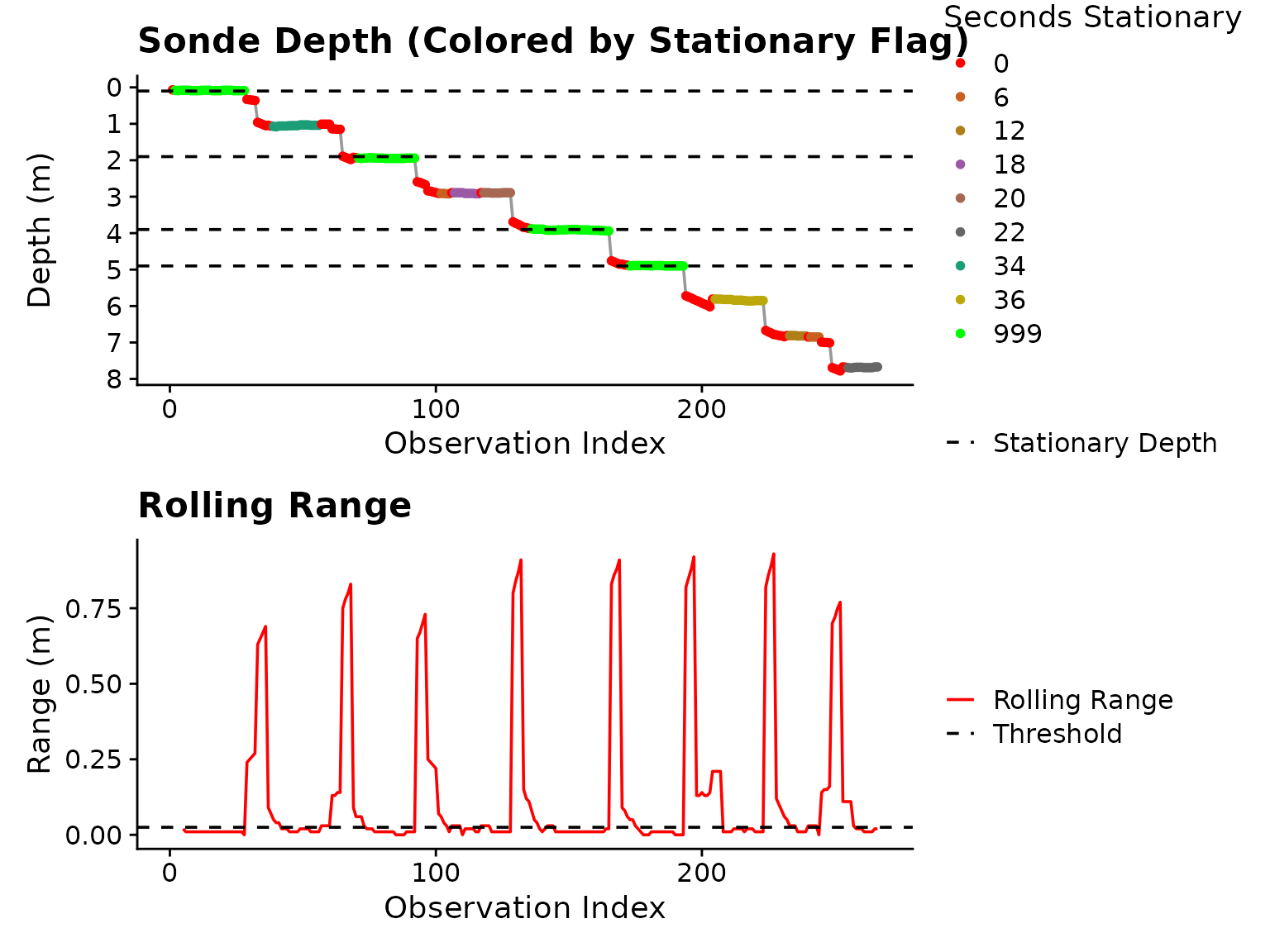 Figure 1: Plot output from
 is_stationary
indicating which stationary depths were extracted (horizontal dashed
lines in top panel).
Once stationary periods are detected, is_stationary
appends stationary_depthas the mean of the stationary
observation depths to the input df. As you can see in the
legend, stationary periods longer than stationary_secs are
flagged with 999, indicating they are fully stationary.
This is critical for downstream use, only
is_stationary_status 999 observations are considered for
stability detection.
In this example, we can see in the bottom panel of Figure
1, that the depth_range_threshold is too strict,
causing splitting of blocks that hover near the same depth.
dat_stationary <-
is_stationary(df = dat_rename,
depth_range_threshold = 0.05, # increased to avoid erroneous splits (this is the default value)
stationary_secs = 40,
rolling_range_secs = 10,
plot = TRUE)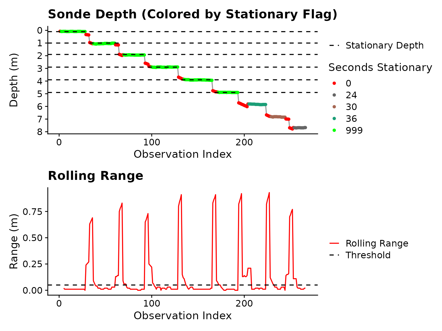 Figure 2: Plot output from
 is_stationary
after adjustment to depth_range_threshold
Now, the blocks are continuous, but it is clear that if we want to
include data from > 5 m, we will have to relax
stationary_secs to allow shorter periods through. If we use
stationary_secs = 24, all blocks to ~ 8.0 m will be
included.
dat_stationary <-
is_stationary(df = dat_rename,
depth_range_threshold = 0.05, # increased to avoid erroneous splits (this is the default value)
stationary_secs = 24,
plot = TRUE)
#> Warning: Inconsistent sampling intervals detected.
#> Dominant interval: 2 secs (99.2% of records) used for `samp_int`.
#> Interval distribution:
#> sampling_interval n
#> 2 263
#> 26 1
#> 66 1
#> Warning: Removed 4 rows containing missing values or values outside the scale range
#> (`geom_line()`).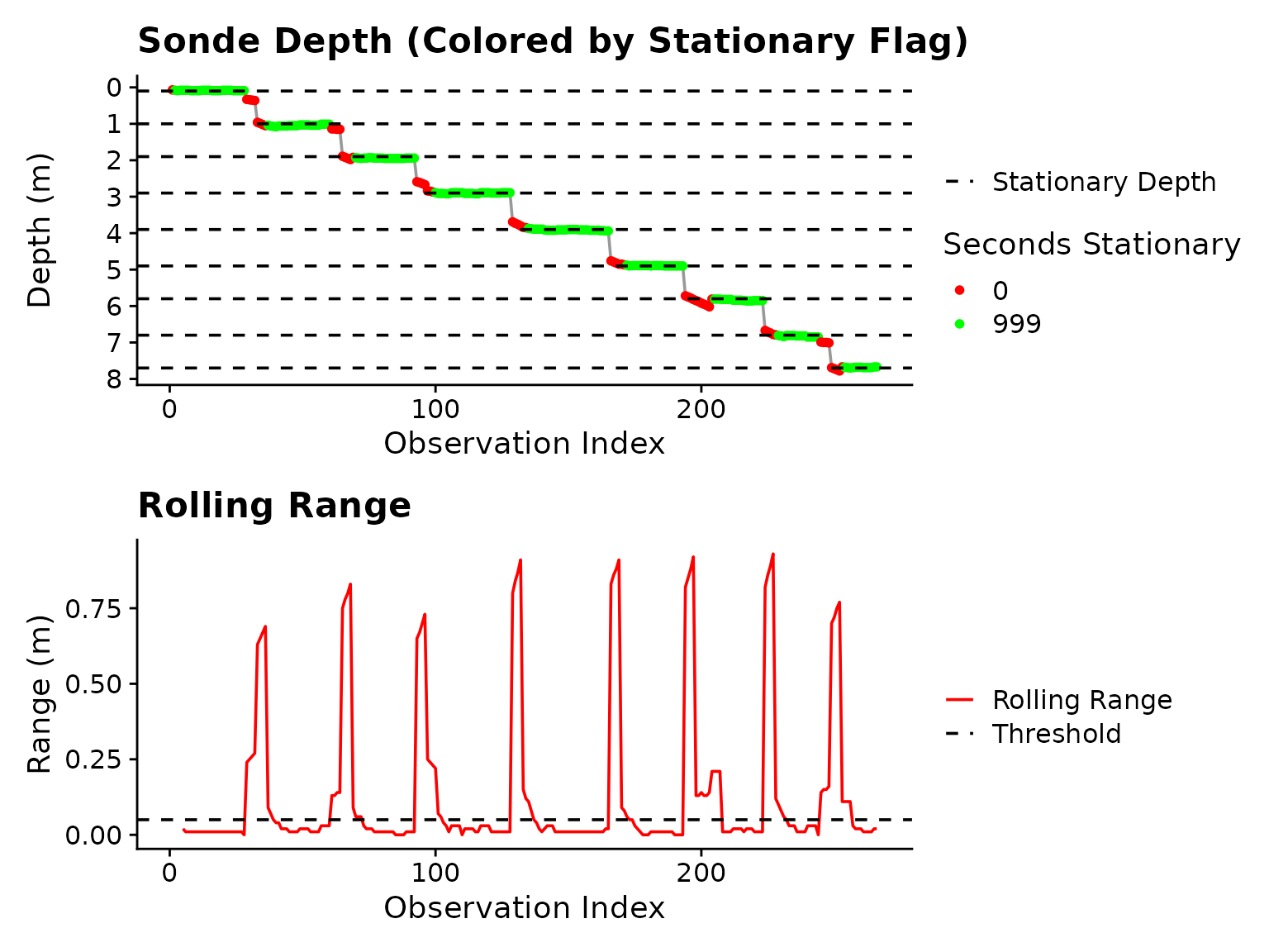 Figure 3: Plot output form
 is_stationary
after adjustment of stationary_secs.
The “Warning: Inconsistent sampling intervals…” is created by an internal helper that extracts sampling interval from the DateTime column. What it’s telling you is that there are inconsistent temporal “jumps” in the data, usually caused by the Troll-Comm glitching. This is only an issue if the “Dominant Interval” is not detected as what it should be (2 seconds in this example is correct). Stationary periods are calculated based on time, so large jumps are not a problem as long as the sonde was held in the same position.
Now we have flagged stationary depth from 0 - 8 meters at ~ 1.0 m intervals.
Step 4: Detect Stable Sensor Data Inside Stationary Blocks
The TROLL_sensor_stable() function handles one column of
sensor data at a time. It is iteratively applied across all parameter
columns within TROLL_profile_compiler using default range
and slope threshold values (stability_ranges). In this
section, the function is applied outside of the compiler to demonstrate
how tuning of TROLL_sensor_stable may be applied for
individual parameters, if necessary.
How Stability Detection Works
At the core, stability detection functions the same across all data parameters:
- Stationary blocks of data are identified using
is_stationary - An initial “settling period” is trimmed from the start of each block
via
settling_secs - Slope and range are calculated across each stationary block independently
- Observations are dropped iteratively from the start of each
stationary block, slope and range are re-calculated on the remainder
until
min_secsof time remains in the stationary block - Once
slope_threshANDrange_threshare met, the remainder of the block is used to calculate the median value
Optical Probes (Turbidity, Chlorophyll, BGA) utilize
all “stationary” data after trimming of stationary_secs due
to optical sensor behavior. A warning is shown if the slope threshold is
exceeded for one of the optical parameters, allowing the user to explore
if there are suspect data at the specific stationary depth output by
TROLL_stable_summary.
Time Series Plots
It may not be intuitive at first to view water column profile data as time series plots, however, by doing so the user is able to visually assess how parameter values are changing through the cast relative to stationary blocks of data, and whether the extracted “stable” data points are representative of reality.
dat_stable <- TROLL_sensor_stable(
df = dat_stationary,
value_col = pH_units,
settling_secs = 10, # Front end trimming of stationary blocks
min_median_secs = 5, # Minimum amount of data retained to calculate median if stability is not detected
slope_thresh = 0.05,
range_thresh = 0.02,
plot = TRUE # Optional plotting toggled ON
)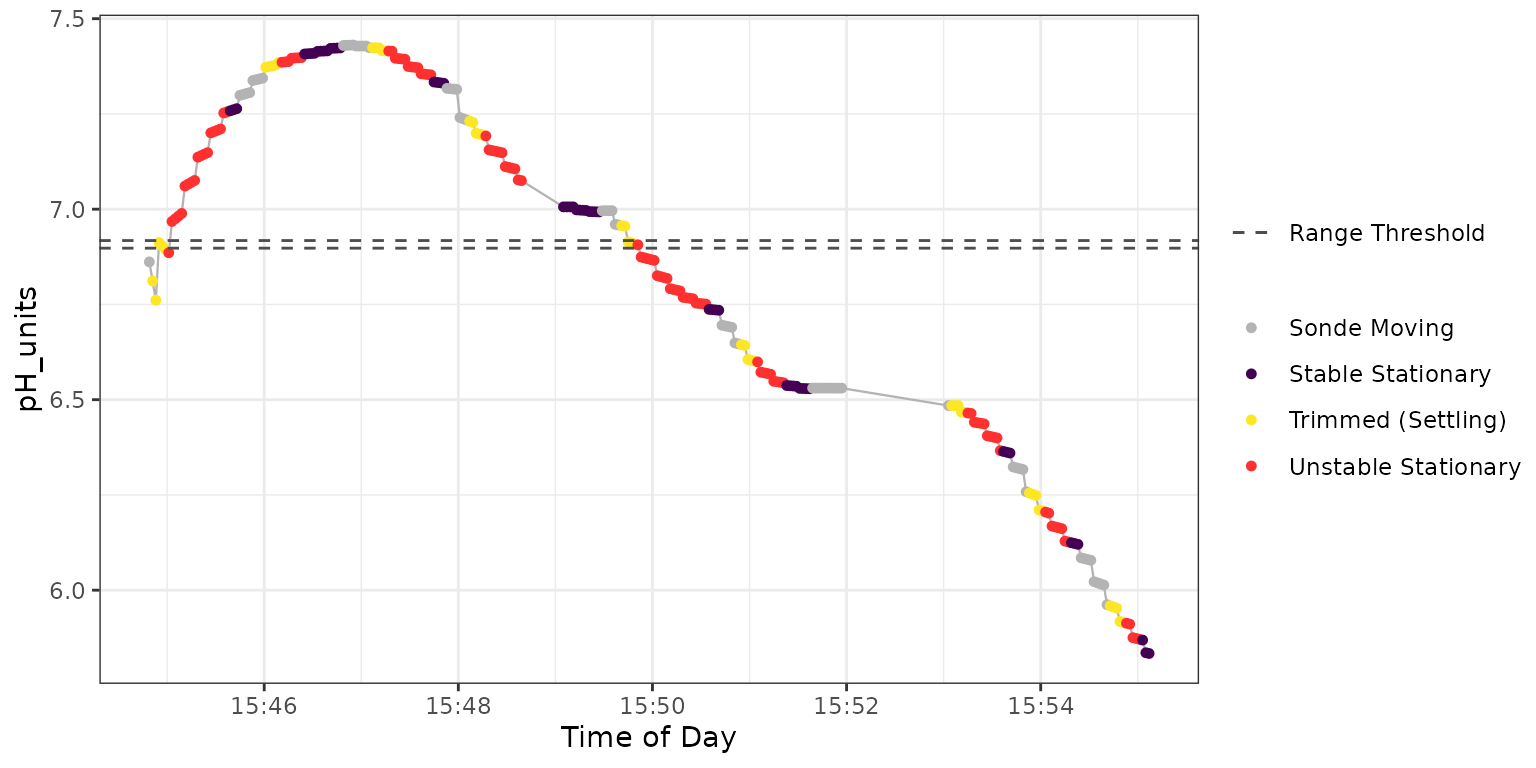 Figure 4: Plot output from
TROLL_sensor_stable for pH.
The horizontal dashed lines represent the range_thresh
value, which can be useful for tuning. The dark purple points are the
extracted “stable” data which are used to calculate the median at each
stationary depth by TROLL_stable_summary.
In Figure 4 an exponential type relationship is apparent across each stationary block of data, with stability occurring late in each block, if at all.
Due to the nature of the parameters being measured, as well as how optical sensors record data, values from optical sensors (turbidity, chlorophyll, BGA) tend to be noisier and not exhibit such exponential changes (Figure 5).
dat_stable <- TROLL_sensor_stable(
df = dat_stationary,
value_col = turbidity_NTU,
settling_secs = 10, # Front end trimming of stationary blocks
min_median_secs = 5, # Minimum amount of data retained to calculate median if stability is not detected
slope_thresh = NULL, # Use defaults
range_thresh = NULL, # Use defaults
plot = TRUE # Optional plotting toggled ON
)
#> Warning in TROLL_sensor_stable(df = dat_stationary, value_col = turbidity_NTU, : turbidity_NTU stability source (turbidity_NTU) slope exceeded threshold at:
#> 2.9 m (0.716 units/min)
#> 6.83 m (-0.554 units/min)
#> 7.68 m (-1.673 units/min)
#>
#> Consider validating data or adjusting trimming.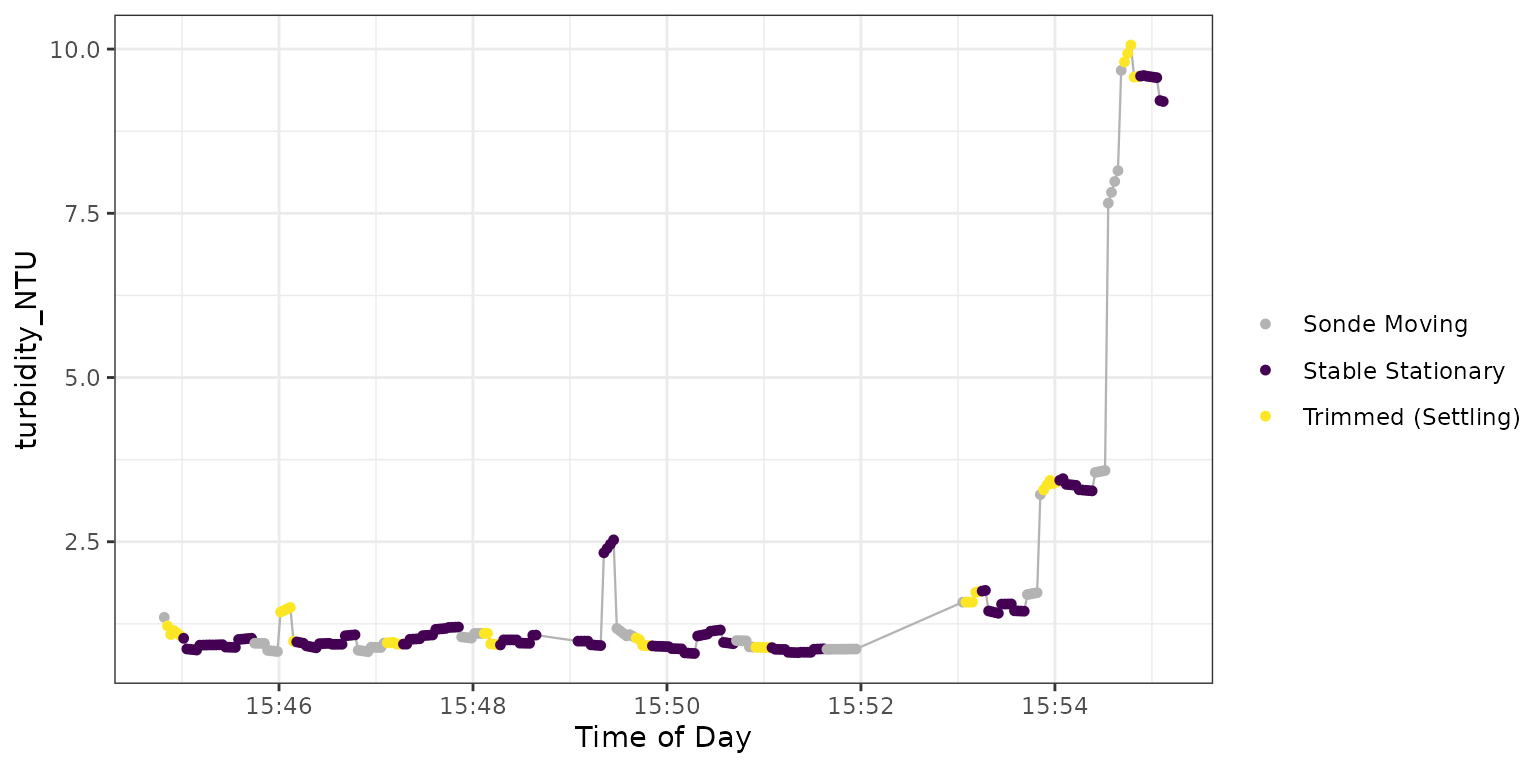 Figure 5: Plot output from
TROLL_sensor_stable for turbidity.
The function here warns us that the slope threshold was exceeded at 3 stationary depths:
- At 2.90 m (the fourth stationary block accounting for depth ~ 0) this is clearly caused by a small number of observations at the tail of the stationary block of ~ 2.4 - 2.5 NTU
- At 6.83 m the data exhibits consistent drift in the negative direction
- At 7.68 m is primarily the result of higher NTU values (on a relative basis such as percent change this would appear less impactful)
There are no range threshold lines in Figure 5 because it is not used for optical sensors.
Derived Parameters
A number of parameters are estimated by the Aqua Troll Sonde using correlations to measured parameters (Table 1).
Table 1: Derived Parameters. “Fully Supported” indicates parameters that have been tested by the developers of this package.
| Parameter | units | Derived From | Stability Source | Fully Supported |
|---|---|---|---|---|
| Total Dissolved Solids | ppt | Conductivity & Temperature | Temperature | NO |
| Total Suspended Solids | ppt | Turbidity & Temperature | Temperature | NO |
| BGA PC concentration | ug/L | Relative Fluorescence | BGA (RFU) | YES |
| BGA PE concentration | ug/L | Relative Fluorescence | BGA (RFU) | YES |
| Chlorophyll concentration | ug/L | Relative Fluorescence | Chlorophyll (RFU) | YES |
| Chlorophyll cell count | cells/mL | Relative Fluorescence | Chlorophyll (RFU) | NO |
| FDOM concentration | ug/L | Relative Fluorescence | Chlorophyll(RFU) | NO |
| Crude Oil Concentration | ug/L | Relative Fluorescence | Chlorophyll (RFU) | NO |
Since derived parameters depend upon measured parameters, detecting
stability is accomplished by simply using stable flags from the
requisite measured parameters (Stability Source in Table
1). If a provided dataframe does not contain the measured
values column, stability detection falls back to the use of the derived
values to determine stability. Since derived parameters are an
estimate based on correlations, best practice is to maintain the
measured data columns used for derivations so that stability
detection may operate on actual measurements. If a derived parameter is
passed to TROLL_sensor_stable(), a message will be printed
to the console when verbose = TRUE, indicating if a
measured parameter was used for stability detection, or if fallback to
the derived parameter was necessary.
# Stability for derived parameter when the measured column is present
derived_dat <-  TROLL_sensor_stable(df = dat_stationary,
                                    value_col = DO_per,
                                    verbose = TRUE,     # Print informative messages to console
                                    plot = FALSE)
#> Derived parameter provided:
#> DO_per
#>  with the measured source column:
#> DO_mgL
#>  utilized for stability detection.
#> Stationary depths at:
#> 0.09
#> 1.04
#> 1.94
#> 2.9
#> 3.91
#> 4.89
#> 5.84
#> 6.83
#> 7.68
#> found in the data

# Fallback to use derived values if measured column is missing
fallback_dat <- TROLL_sensor_stable(df = dat_stationary |> dplyr::select(-DO_mgL),
                                    value_col = DO_per,
                                    verbose = TRUE,
                                    plot = FALSE)
#> Stability detection for DO_per is based on derived values because source column DO_mgL is missing.
#> Stationary depths at:
#> 0.09
#> 1.04
#> 1.94
#> 2.9
#> 3.91
#> 4.89
#> 5.84
#> 6.83
#> 7.68
#> found in the data
Step 5: Summarize Stable Data
With data flagged as stable in hand, the
TROLL_stable_summary function compiles the output into a
single value (default = median) for each stationary depth. This is
carried out internally in TROLL_profile_compiler when
summarize_data is set to TRUE. For
demonstration here we compile the summary data for turbidity used in
Figure 5.
dat_summary <- TROLL_stable_summary(
  df = dat_stable,
  group_col = stationary_depth
) |>
  dplyr::select(stationary_depth, turbidity_NTU)
#> Warning: There was 1 warning in `dplyr::summarise()`.
#> ℹ In argument: `dplyr::across(...)`.
#> ℹ In group 1: `stationary_depth = 0.085`.
#> Caused by warning:
#> ! `cur_data()` was deprecated in dplyr 1.1.0.
#> ℹ Please use `pick()` instead.
#> ℹ The deprecated feature was likely used in the ImportUtils package.
#>   Please report the issue to the authors.
dat_summary
#> # A tibble: 9 × 2
#>   stationary_depth turbidity_NTU
#>              <dbl>         <dbl>
#> 1            0.085         0.928
#> 2            1.04          0.950
#> 3            1.94          1.08
#> 4            2.9           0.987
#> 5            3.91          0.912
#> 6            4.89          0.860
#> 7            5.84          1.45
#> 8            6.83          3.36
#> 9            7.68          9.58
Step 6: Putting it all Together
The TROLL_profile_compiler function is a high level
wrapper that automatically detects parameters using the
troll_colname_dictionary and iterates over them with
TROLL_sensor_stable to provide summarized data from an
entire AquaTroll sonde cast. Inputs to the compiler are named to
indicate which of the other package functions they relate to:
- prefix “stn_” is associated with inputs to
is_stationary - prefix “stbl_” is associated with input to
TROLL_sensor_stable
The output from the compiler is either:
-
A list of length (2) if
summarize_datais set toTRUEThe first list element is named “Flagged_Data”, and is the raw input dataframe with a “_stable” flag appended to each parameter column.
The second list element is the summary output from
TROLL_stable_summary.
Instead of timeseries plots, the compiler function outputs classical
“profile” plots for each of the core parameters in the data when
plot = c(Final = TRUE).
Updating Inputs to the Compiler Based on Tuning Results
If the default values for any of the inputs needs to be tuned, they can updated:
Table 2: Input naming conventions among package functions.
| TROLL_profile_compiler | Other Package Function | Other Function Input |
|---|---|---|
| stn_depthrange | is_stationary() | depth_range_threshold |
| stn_secs | is_stationary() | stationary_secs |
| stn_rollwindow_secs | is_stationary() | rolling_range_secs |
| stbl_settle_secs | TROLL_sensor_stable() | settling_secs |
| stbl_min_secs | TROLL_sensor_stable() | min_median_secs |
| stbl_range_thresholds | TROLL_sensor_stable() | range_thresh |
Default values for individual range_thresh and
slope_thresh by parameter are given by
stability_ranges:
#> # A tibble: 16 × 3
#>    param                   range   slope
#>    <chr>                   <dbl>   <dbl>
#>  1 sp_conductivity_uScm     0.5     1
#>  2 temperature_C            0.15    0.25
#>  3 pH_units                 0.1     0.05
#>  4 DO_mgL                   0.15    0.15
#>  5 turbidity_NTU            4       0.5
#>  6 chlorophyll_RFU          1       0.5
#>  7 bga_fluorescence_RFU     1       0.5
#>  8 ORP_mv                  10       1
#>  9 DO_per                   3       5
#> 10 chlorophyll_ugL          1.5     1
#> 11 bga_fluorescence_ugL     1       0.75
#> 12 chlorophyll_cells     5000    5000
#> 13 total_diss_solids_ppt   15      10
#> 14 total_susp_solids_ppt   20      15
#> 15 FDOM                     1       0.5
#> 16 crude_oil               10       5
These may be updated by passing a named numeric vector. If we want to
relax the range_thresh for dissolved oxygen and pH as an
example:
# Create a named vector of new range threshold values
custom_ranges <- c('DO_mgL' = 0.2, 'pH_units' = 0.15)

dat_final <- TROLL_profile_compiler(
  path = file_location_path,
  stn_depthrange = 0.05,
  stn_secs = 24,                                   # Note use of value from tuning above
  stbl_range_thresholds = custom_ranges,           # Provide updated custom ranges
  summarize_data = TRUE,                           # Output will be a list w/ both flagged and summary data
  plot = c(Final = FALSE, Stationary = FALSE)
)
Currently updating of slope thresholds is not allowed
If summarize_data is FALSE, output will
just return the raw dataframe with a “_stable” flag column for each
parameter. Flagged_Data is always returned, but the
Summary_Data can be extracted from the output list when
summarize_data = TRUE:
flag_data <- dat_final$Flagged_Data
summary <- dat_final$Summary_Data
Table 2: Example of $Summary_Data from
the compiler function output.
| stationary_depth | sp_conductivity_uScm | temperature_C | pH_units | DO_mgL | DO_per | chlorophyll_RFU | turbidity_NTU | bga_fluorescence_RFU |
|---|---|---|---|---|---|---|---|---|
| 0.085 | 66.8068 | 18.0236 | 7.2610 | 9.8488 | 107.8445 | 0.0925 | 0.9281 | 0.0298 |
| 1.042 | 66.5640 | 18.0551 | 7.4148 | 9.8603 | 108.1485 | 0.8366 | 0.9497 | 0.0297 |
| 1.943 | 66.3416 | 17.5420 | 7.3321 | 9.6794 | 105.0327 | 1.4116 | 1.0790 | 0.0335 |
| 2.900 | 66.7060 | 16.0662 | 6.9974 | 9.1063 | 95.8559 | 1.8915 | 0.9871 | 0.0550 |
| 3.910 | 65.6661 | 15.2921 | 6.7359 | 8.0189 | 82.8336 | 1.6172 | 0.9122 | 0.0358 |
| 4.894 | 67.1874 | 12.6911 | 6.5325 | 6.4276 | 62.6799 | 0.1776 | 0.8601 | 0.0150 |
| 5.837 | 66.8931 | 10.6287 | 6.3620 | 5.0798 | 47.2309 | 0.0623 | 1.4473 | 0.0078 |
| 6.827 | 66.9843 | 9.8301 | 6.1224 | 4.0520 | 36.9335 | 0.0342 | 3.3588 | 0.0076 |
| 7.685 | 68.8675 | 9.5200 | 5.8358 | 2.3769 | 21.4933 | 0.0357 | 9.5760 | 0.0139 |
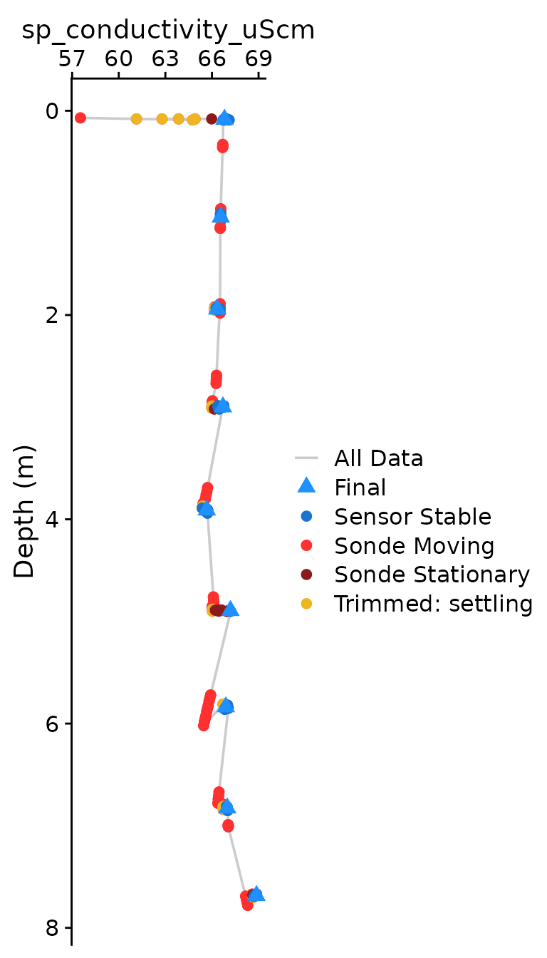
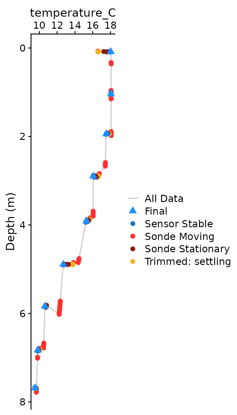
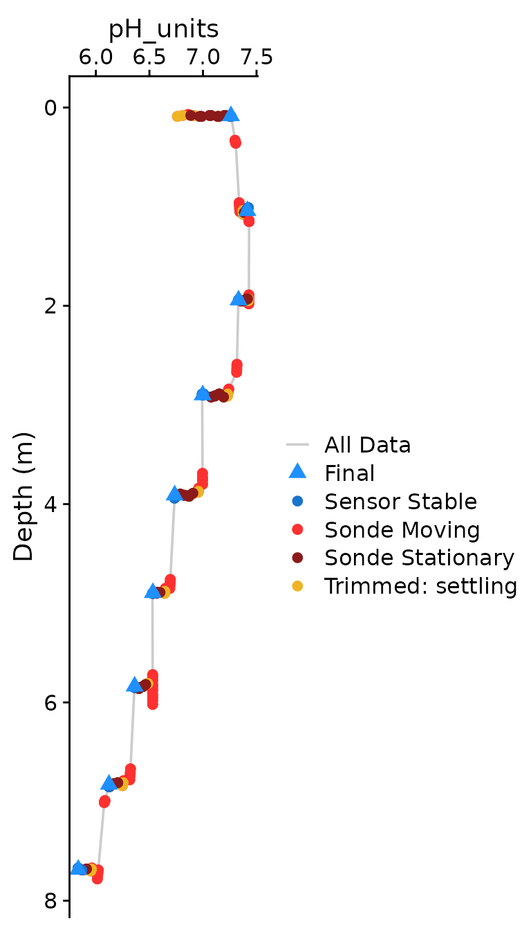
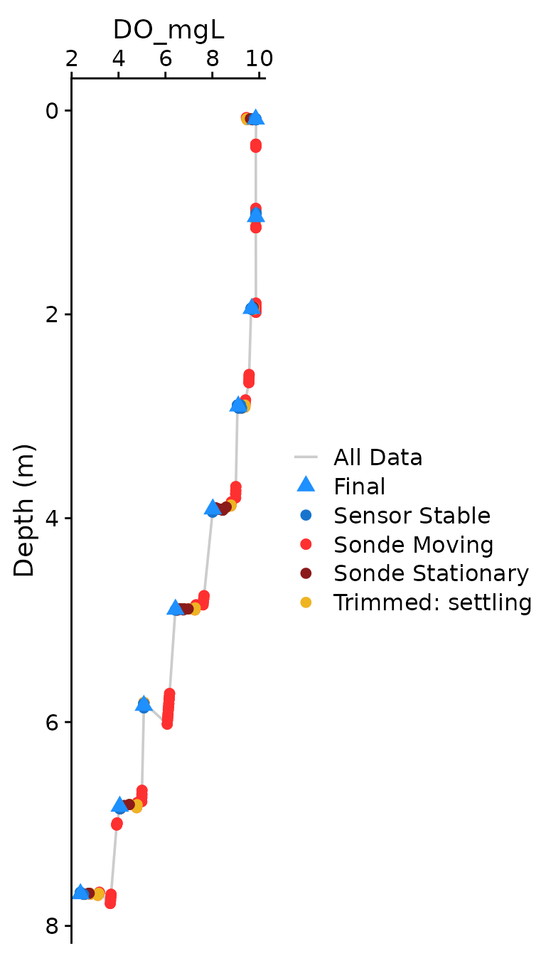
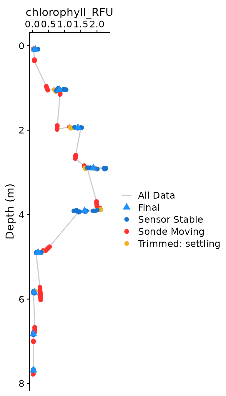
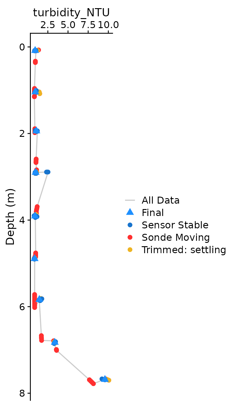
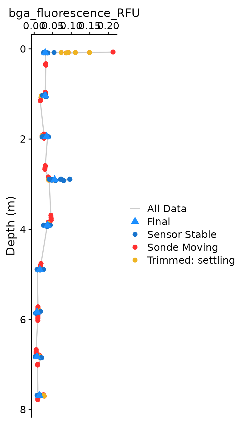
The optional plotting should be used to visually ensure that each
parameter was compiled as expected. The plots shown below are the
classical view of profile data, with data values on the x axis and depth
on the y-axis. Optional plotting is toggled with
plot = c(Final = TRUE),
plot = c(Final = TRUE, Stationary = TRUE) (to show the
stationary plot like Figure 3), or
plot = TRUE (toggles both plots ON).
If any individual parameter looks incorrect, it is recommended to
move outside of TROLL_profile_compiler and work in the
individual workflow to tune, and bring those values back to the
wrapper.